Structured Linear CDEs
Introduction
This post is an introduction to Structured Linear Controlled Differential Equations (SLiCEs): a framework for sequence models that balance expressivity with efficient parallel-in-time computation by using structured, input-dependent state-transition matrices. This framework was introduced in our NeurIPS 2025 spotlight paper. We start by outlining how SLiCEs connect to linear recurrent neural networks and linear neural controlled differential equations, before motivating why expressivity matters. We then introduce SLiCEs and compare their properties, finishing with some empirical results.
Linear Recurrent Neural Networks
Given observations from a time series $\{x_i\}_{i=0}^n$, an RNN has the generic form
$$ h_{i+1} = g_\theta(h_i, x_i). $$
Linear RNNs further restrict to
$$ h_{i+1} = W_\theta h_i + B_\theta x_i = h_i + A_\theta h_i + B_\theta x_i, $$
where $W_\theta = I + A_\theta \in \mathbb{R}^{d_h \times d_h}$ and $B_\theta \in \mathbb{R}^{d_h \times d_x}$. Just as residual networks can be seen as an Euler discretisation of a Neural ODE, the linear RNN is an Euler discretisation of
$$ \frac{\mathrm{d}h_s}{\mathrm{d}s} = A_\theta h_s + B_\theta X_s, $$
where $X_s$ is an interpolation of the input sequence $\{x_i\}_{i=0}^n$. Due to the similarity to classical state-space models, a popular class of linear RNNs are known as structured state-space models (SSMs). The simple recurrence allows for parallelisation via associative scans or convolution. However, linear RNNs are not very expressive, which motivates making the state-transition matrix depend on the input:
$$ \frac{\mathrm{d}h_s}{\mathrm{d}s} = A_\theta(X_s) h_s + B_\theta X_s. $$
For example, Mamba takes this approach. Although no longer time invariant, these models can still be computed in parallel using associative scans. A natural question is: How expressive are input-dependent linear RNNs?
Quick Tangent on Names
These models are often called (input-dependent) linear RNNs, with many variants detailed in Table 2 of this paper. Since the update has multiplicative interactions between $X_s$ and $h_s$, they are not linear in $(h_s, X_s)$. A more descriptive term would be linear multiplicative RNNs or linear 2-RNNs, both of which are nonlinear RNNs where the matrix multiplying the hidden state depends linearly on the input. See here and here for examples. These names would emphasise that “linear” refers to the absence of pointwise nonlinearities on the hidden state update.
Linear Neural Controlled Differential Equations
Linear neural controlled differential equations (LNCDEs) are continuous-time models where the state-transition depends linearly on the increments of the input:
$$ \mathrm{d}h_s = \sum_{j=1}^{d_\omega} A^j_\theta\, h_s\, \mathrm{d}\omega^{X, j}_s + B_\theta\, \mathrm{d}\xi^{X}_s. $$
Taking $\mathrm{d}\omega^{X,j}_s = X^j_s\, \mathrm{d}s$ and $\mathrm{d}\xi^X_s = X_s\, \mathrm{d}s$, we recover the input-dependent linear RNN while restricting $A_\theta$ to be linear in $X_s$. Thus, LNCDEs are the continuous-time analogue of linear 2-RNNs. As shown in our NeurIPS 2024 paper, linear dependence in the state transition is sufficient for maximal expressivity (universality), which answers how expressive generic input-dependent linear RNNs are. However, S4D and Mamba are special cases of LNCDEs with diagonal $A^j_\theta$; this restriction is computationally efficient but limits expressivity.
A Simple Parity Example
Consider a stream of bits $x_0,x_1,x_2,\dots\in\{0,1\}$ and the parity label
$$ p_n = S_n \bmod 2 \in \{0,1\}, \quad S_n = \sum_{k=0}^{n-1} x_k. $$
Whenever $x_i=1$ the label flips; if $x_i=0$ the label stays the same. Take
$$ \frac{\mathrm{d}h_s}{\mathrm{d}s} = A_\theta X_s h_s, $$
with $h_s\in\mathbb{R}^2$, piecewise constant $X_s=x_i$ for $s\in[i,i+1)$, and diagonal $A_\theta$. Then
$$ h_{n+1} = \exp\left(\begin{bmatrix} a_1 & 0 \\ 0 & a_2\end{bmatrix} x_n\right) h_n, \qquad h_n^{i}=h_0^{i} e^{a_i S_n},\ i=1,2. $$
With a linear readout $r=(r_1,r_2)^\top$ and monotone $\phi$:
$$ \hat p_n = \phi\Big(r^\top h_n\Big) = \phi\Big(c_1 e^{a_1 S_n} + c_2 e^{a_2 S_n}\Big) = \phi\big(f(S_n)\big), \quad c_i=r_i h_0^{i}. $$
Since $f(S)$ has at most one turning point and $\phi$ is monotone, $\hat p_n$ crosses any fixed threshold at most twice, while $p_n$ flips every time $S_n$ increases by one. Therefore, a diagonal $A$ cannot realise parity on arbitrarily long input.
Now take $A = \begin{pmatrix} 0 & \pi \\ -\pi & 0 \end{pmatrix}$. Then
$$ \exp(A x_{n}) = \begin{pmatrix}1 & 0 \\ 0 & 1\end{pmatrix} \text{ if } x_{n}=0, \quad \exp(A x_{n}) = \begin{pmatrix}-1 & 0 \\ 0 & -1\end{pmatrix} \text{ if } x_{n}=1, $$
so $h_{n+1} = (-1)^{x_{n}} h_n$ and hence $h_n = (-1)^{S_n} h_0$. With $r=(1,0)^\top$, $h_0^{(1)}=1$, and $\phi(s) = \big(1-\operatorname{sign}(s)\big)/2$,
$$ \hat p_n = \frac{1-\operatorname{sign}\big((-1)^{S_n}\big)}{2} = S_n \bmod 2 = p_n. $$
Therefore, a dense matrix can solve parity exactly with $d_h=2$.
However, moving from diagonal to dense matrices is impractical for large $d_h$: parameter count and compute grow from $\mathcal{O}(d_\omega d_h)$ to $\mathcal{O}(d_\omega d_h^2)$. This motivates structured alternatives that balance expressivity and efficiency, leading us to SLiCEs.
Structured Linear Neural Controlled Differential Equations
SLiCEs replace the dense matrices of an LNCDE with structured variants that preserve expressivity while being computationally cheaper. Our paper proposes:
- DPLR-SLiCE: $A^i_\theta = D^i_\theta + \sum_{j=1}^r u^{i,j}_{\theta} (v^{i,j}_{\theta})^\top$. Includes DeltaNet, DeltaProduct, and Gated DeltaNet.
- BD-SLiCE: $A^i_\theta = \mathrm{BlockDiag}(B^i_{\theta,1},\ldots,B^i_{\theta,k})$. Includes block-diagonal input-dependent linear RNN.
- S-SLiCE: $A^i_\theta$ is sparse with $\mathcal{O}(d_h^{1+\epsilon})$ non-zeros for some $\epsilon>0$.
- WH-SLiCE: $A^i_\theta = H\, D^i_\theta$ for a (normalised) Hadamard matrix $H$.
All four of these choices are maximally expressive (universal), as shown for DPLR-SLiCE in this paper, and shown for BD, sparse, and WH-SLiCE in our paper.
Comparison of SLiCEs
The opening figure visualises six possible structures: dense LNCDE (DE-LNCDE), diagonal SLiCE (D-SLiCE), diagonal-plus-low-rank (DPLR-SLiCE), sparse (S-SLiCE), Walsh–Hadamard (WH-SLiCE), and block-diagonal (BD-SLiCE). The table below compares parameter count, computational cost, and whether each is maximally expressive (Max. Exp.). Here $d_h$ is hidden size, $n$ sequence length, $b_j$ BD block sizes, $r$ DPLR rank, $\epsilon$ sparse exponent, and we take $d_\omega=d_h$ for simplicity. Parallel cost is measured as $\mathcal{O}(\text{scan depth, cost per composition})$ when using a parallel associative scan.
| Model | Parameters | Recurrent Cost | Parallel Cost | Max. Exp. |
|---|---|---|---|---|
| DE-LNCDE | $\mathcal{O}(d_h^3)$ | $\mathcal{O}(n d_h^3)$ | $\mathcal{O}(\log n, d_h^3)$ | Yes |
| D-SLiCE | $\mathcal{O}(d_h^2)$ | $\mathcal{O}(n d_h^2)$ | $\mathcal{O}(\log n, d_h^2)$ | No |
| DPLR-SLiCE | $\mathcal{O}(r d_h^2)$ | $\mathcal{O}(n r d_h^2)$ | $\mathcal{O}(\log n, d_h^3)$ | Yes |
| S-SLiCE | $\mathcal{O}(d_h^{2+\epsilon})$ | $\mathcal{O}(n d_h^{2+\epsilon})$ | $\mathcal{O}(\log n, d_h^3)$ | Yes |
| WH-SLiCE | $\mathcal{O}(d_h^2)$ | $\mathcal{O}(n d_h^2)$ | $\mathcal{O}(\log n, d_h^3)$ | Yes |
| BD-SLiCE | $\mathcal{O}\!\left(d_h \sum_j b_j^2\right)$ | $\mathcal{O}\!\left(n d_h \sum_j b_j^2\right)$ | $\mathcal{O}\!\left(\log n, d_h \sum_j b_j^2\right)$ | Yes |
Parallel Computation
Block-diagonal matrices are closed under multiplication, so the parallel associative scan preserves their structure. For DPLR, sparse, and WH, compositions destroy structure, yielding an effective $\mathcal{O}(d_h^3)$ cost per composition. Another important consideration is that for large hidden sizes, scans can incur high I/O costs, which reduces their practical benefit. DeltaNet mitigates this using a chunk-wise algorithm tailored for diagonal-plus-low-rank matrices; see this blog post. Because chunk-wise methods also apply to diagonal matrices, BD-SLiCE with a mostly diagonal structure ($b_i=1$ for $i=1,\ldots,k-1$) plus a small dense block ($b_k=b$) is an attractive option when $d_h$ is large. This variant can leverage chunk-wise updates for the diagonal part and scans for the dense part. We refer to this structure as diagonal–dense SLiCE (D-DE-SLiCE).
Empirical Results
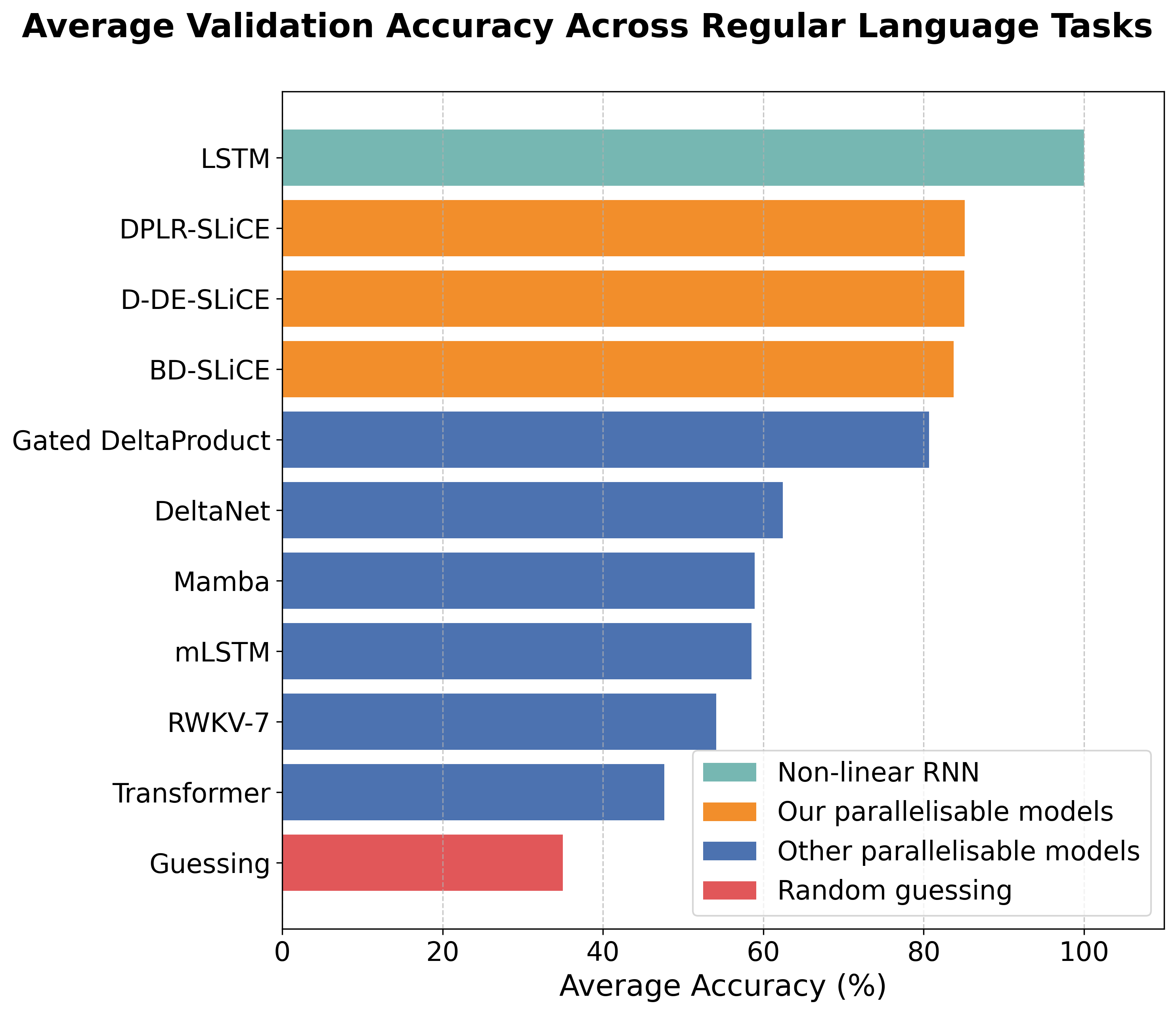
Two highlights. First, DPLR, BD, and D-DE achieve strong length generalisation on regular language tasks from the Formal Language Benchmark, outperforming all parallel-in-time baselines we considered.
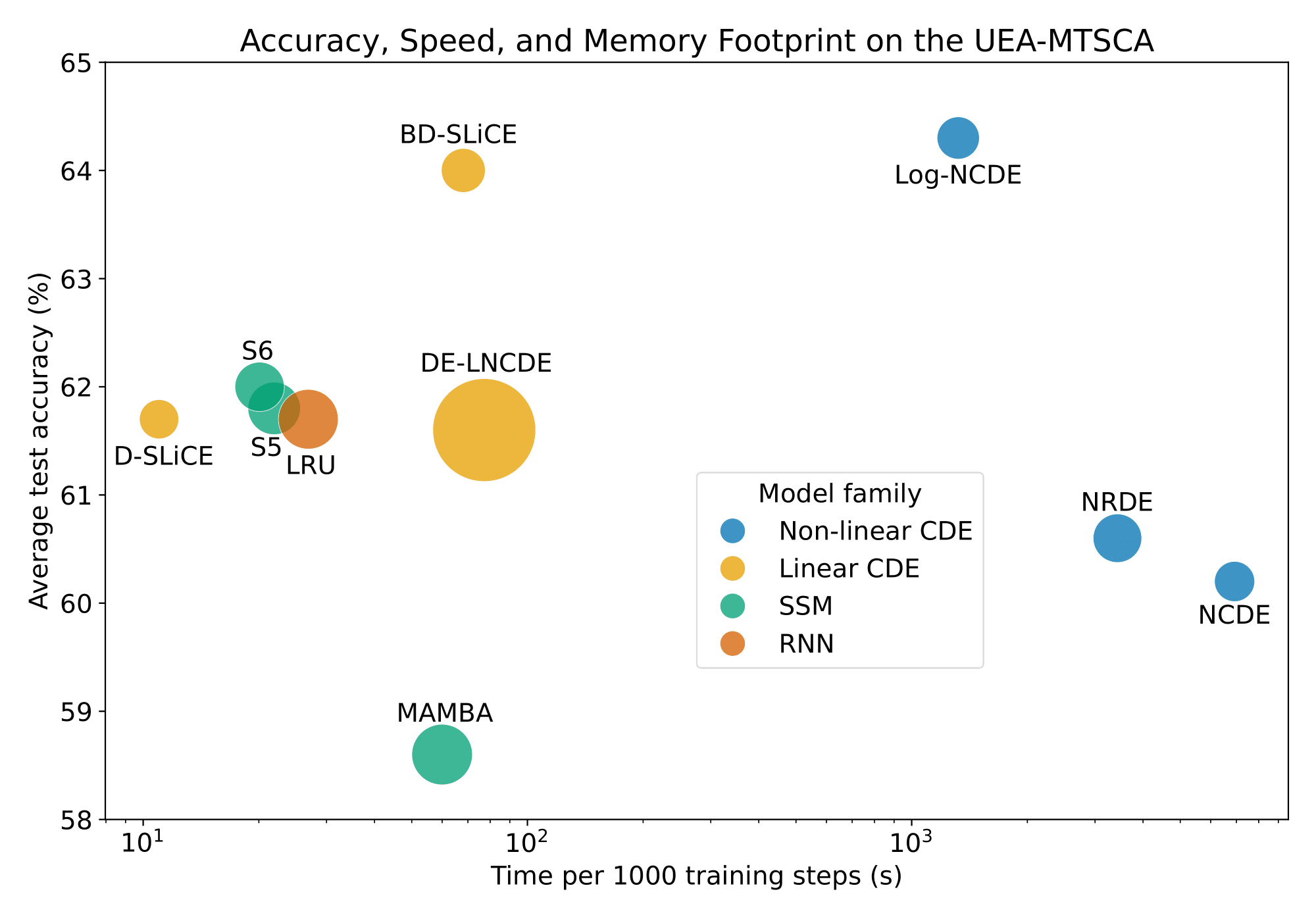
Second, replacing the nonlinear vector field of a Log-NCDE with a block-diagonal linear field (BD-SLiCE) gives the same average test accuracy with a $20\times$ reduction in average time per training step over six datasets from the UEA Multivariate Time Series Classification Archive.
Conclusion
SLiCEs provide a framework for understanding structured, input-dependent state-transition matrices that are both maximally expressive and parallel-in-time. If you want to keep learning more about them, further details, proofs of theoretical claims, and thorough experiments can be found in our paper. If you want to start using them, we have released open-source implementations in both PyTorch and JAX.
As for what is next, we are currently working on efficient implementations so that we can scale SLiCEs to the billion-parameter regime. We are also interested in exploring other structured matrices that fit within the SLiCE framework, so please reach out if you have any ideas!
Thanks for reading!